August 10, 2026

CARDQN: teaching a cautious trading agent to read the room

How to make a robust agent less scared — without making it reckless.

A robust trading agent hedges against the worst plausible market move every day. That’s safe — it won’t blow up — but on a drifting asset like the S&P 500 it ends 30 years at about 2–3×, while buy-and-hold nets 9.5×. Safe, and leaving a fortune on the table.

CARDQN (Context-Aware Distributionally Robust Deep Q-Learning) teaches that agent to read the room: stay defensive when the market is uncertain, relax the hedge when conditions are clear and the model can be trusted — same robustness guarantee where it matters, far less wasted caution where it doesn’t. No prior knowledge assumed. Code · paper (PDF).

Table of contents

1. Why reinforcement learning? (and why not just “solve” Bellman)
2. The reference cloud ν — representing the market model
3. Distributional robustness: planning for the worst
4. CARDQN: making the hedge read the room
   • 4.1 Why one global ball is too cautious
   • 4.2 The regime tag τ
   • 4.3 The fidelity score — entropy, and why we score it out-of-sample
   • 4.4 Adaptive radius and reference — and where they come from
   • 4.5 The target, and a proposed blend
5. How it all fits together
6. Does it actually work?
7. Takeaways

1. Why reinforcement learning? (and why not just “solve” Bellman)

The agent learns the action-value function $Q(x,a)$ — the expected total future reward of taking action $a$ in state $x$. With a good $Q$, the policy is trivial: pick the highest-$Q$ action each step. $Q$ must satisfy the Bellman equation:

the immediate reward $r$ plus (discounted by $\gamma$) the best you can do from the next state $X’$. You can’t just solve this for $Q^*$, for three reasons:

1. The state space is enormous — $x$ is a window of recent returns plus your position, a point in a high-dimensional continuous space; you can’t tabulate $Q$ at every state.
2. The transition model is unknown — the expectation is over $X’$, but you don’t have the true $P(X’\mid x,a)$, only data, so you can’t even evaluate the right-hand side.
3. It’s self-referential — $Q^*$ appears on both sides; it’s a fixed-point condition, not a formula you rearrange.

So we approximate $Q$ with a neural network $Q_\theta$ and learn it from experience (Q-learning / DQN): collect transitions $(x,a,r,x’)$; form a target $y = r + \gamma\max_b Q_\theta(x’,b)$; nudge $\theta$ by gradient descent so $Q_\theta(x,a)\to y$. Over enough samples $Q_\theta\to Q^*$. RL is how you learn the Bellman fixed point approximately, from samples, with a function approximator.

For trading: state $x$ = window of past log-returns + position; action $a$ = portfolio weight (cash ↔ all in); reward $r$ = change in log-wealth (so rewards telescope into total log-return).

2. The reference cloud ν — representing the market model

The Bellman expectation needs a model $\hat P$ of the next return. We never write a closed form; we represent it as a cloud of samples

where $\nu$ is a sampling distribution — a prior over tomorrow’s return — and the cloud is the empirical model: $\mathbb{E}_{\hat P}[f]\approx\frac{1}{N}\sum_i f(z_i)$ (Monte-Carlo). Here $\nu$ is a heavy-tailed Student-$t$: real returns have fat tails (crashes), and a heavy-tailed cloud makes the agent rehearse the nasty scenarios a Gaussian would ignore. Think of $\nu$ as a prior over the worst case — it shapes which adverse futures the agent considers. (The worst-case optimisation is also solved sample-wise over this cloud, via the Sinkhorn iterations in §3.)

3. Distributional robustness: planning for the worst

$\hat P$ is only an estimate — trust it completely and your $Q$ is brittle the moment reality differs. Distributionally robust deep Q-learning (RDQN) refuses to commit: consider every model close to $\hat P$ and plan for the worst.

“Close” = optimal transport (Wasserstein). Draw an ambiguity ball of radius $\varepsilon$:

and take the worst case over it:

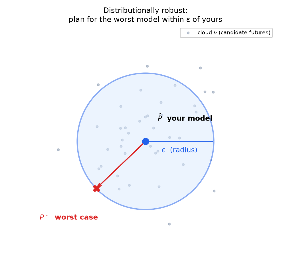
$\hat P$ sits at the centre; the ball holds every model you can’t rule out; an adversary picks the nastiest, $P^\star$, on the boundary; you act as if $P^\star$ were true. $\varepsilon$ is your distrust budget — bigger = more robust, more pessimistic. The inner min is computable: with an entropy penalty it becomes a smooth dual solved by Sinkhorn iterations over the cloud.

4. CARDQN: making the hedge read the room

CARDQN extends RDQN with four additions, each building on the last:

• A regime tag $\tau$ (§4.2) — past-only label of the current market (trend, volatility, position; 27 regimes).
• A fidelity score $\varphi$ (§4.3) — out-of-sample measure of how reliably the model predicts each regime.
• An adaptive radius $\tilde\varepsilon$ and reference $\tilde P$ (§4.4) — the ball tightens where $\varphi$ is high, stays wide where it’s low.
• A Bellman-target blend (§4.5) — de-hedges toward the nominal target in favorable regimes (proposed, not yet validated).

4.1 Why one global ball is too cautious

Taking a min over the ball is pessimistic — on a drifting asset the agent under-invests. RDQN compounds this: it pools every regime into one model $\hat P$ with one radius $\varepsilon$, so the margin is sized for the hardest regime and applied everywhere, even in calm uptrends. CARDQN’s fix: a different ball per regime — tight where you can trust the model, wide where you can’t.

4.2 The regime tag τ

CARDQN’s first move is to label the regime. The context tag

has three components, each three levels → $|\mathcal{T}| = 3^{3} = \mathbf{27}$ regimes, all computed past-only from the last $k$ log-returns ($k=w=20$, ~one month).

Trend — sign of the mean consecutive difference of recent returns: up, down, or sideways?

Volatility — RMS of recent returns, bucketed low/mid/high by frozen terciles ($q_{33},q_{67}$) of the full-history vol distribution (computed once, so labels don’t drift as the dataset grows): calm or turbulent, on a stable scale?

Position — is today’s return near a recent extreme? ($\kappa=0.5$ window-std band; near an extreme often signals reversal.)

Cell index: $\,\tau_{\text{trend}}!\cdot 9 + \tau_{\text{vol}}!\cdot 3 + \tau_{\text{pos}}\in{0,\dots,26}$. $\tau$ underpins everything that follows: fidelity (§4.3), radius/reference (§4.4), the blend (§4.5).

4.3 The fidelity score — entropy, and why we score it out-of-sample

Not all regimes are equal. The fidelity $\varphi(\tau)\in[0,1]$ says how much to trust the model in regime $\tau$. Its core is the entropy of the regime’s next-return distribution — its unpredictability:

(bin the regime’s next returns into $B$ bins; $p_k$ = fraction in bin $k$; low $H_\tau$ = concentrated = predictable, high = spread = unpredictable). Then

two factors: enough samples ($N_\tau$ vs floor $N_{\min}$) and predictability ($1-H_\tau/\log B\in[0,1]$, normalised by max entropy $\log B$). $\varphi$ is high only when the regime is both well-sampled and predictable.

But $H_\tau$ there is not the in-sample entropy. The obvious estimate — build the histogram from the regime’s transitions, plug into $-\sum p_k\log p_k$ — is in-sample: you score on the same data you fit. CARDQN uses the out-of-sample cross-entropy instead. Split each regime’s transitions into a fit half and a score half; fit $\hat p_{\text{fit}}$ on one, score on the other:

— if I built my model on half the data, how surprised am I by the other half? Crucially $H^{\text{OOS}} = H + \mathrm{KL}(p_{\text{true}}\,|\,\hat p_{\text{fit}}) \ge H$: an overfit $\hat p$ (memorised noise) assigns tiny probability to held-out returns → inflates $H^{\text{OOS}}$ → deflates $\varphi$. Score in-sample and the opposite happens: an overfit regime looks great → tiny $H$ → inflated $\varphi$ → CARDQN tightens the ball (§4.4) on a model that doesn’t generalise → the agent trades on a wrong model. This is precision vs accuracy — in-sample measures precision (fits the data you have); out-of-sample measures accuracy (predicts data you don’t). We need accuracy. So $H_\tau$ in the formula is the cross-entropy whenever a regime has enough transitions to split (tiny regimes fall back in-sample, but $N_\tau/N_{\min}$ already drives their $\varphi\to 0$).

4.4 Adaptive radius and reference — and where they come from

The ball is now regime-dependent. Radius shrinks where fidelity is high:

and the reference (ball centre) blends from the global model toward the regime’s own dynamics:

Both are clouds, drawn differently:

• $P_{\text{global}}$ — the safe, regime-agnostic prior: drawn once from $\nu$ (the Student-$t$ of §2), a fixed $N$-quantile grid; never depends on regime or training data; also the fallback for data-poor regimes.
• $P_{\text{context}}(\tau)$ — what tends to happen after this regime: drawn from the regime’s own next returns in the replay buffer (a quantile grid at the same levels as the global one, fit to this regime).

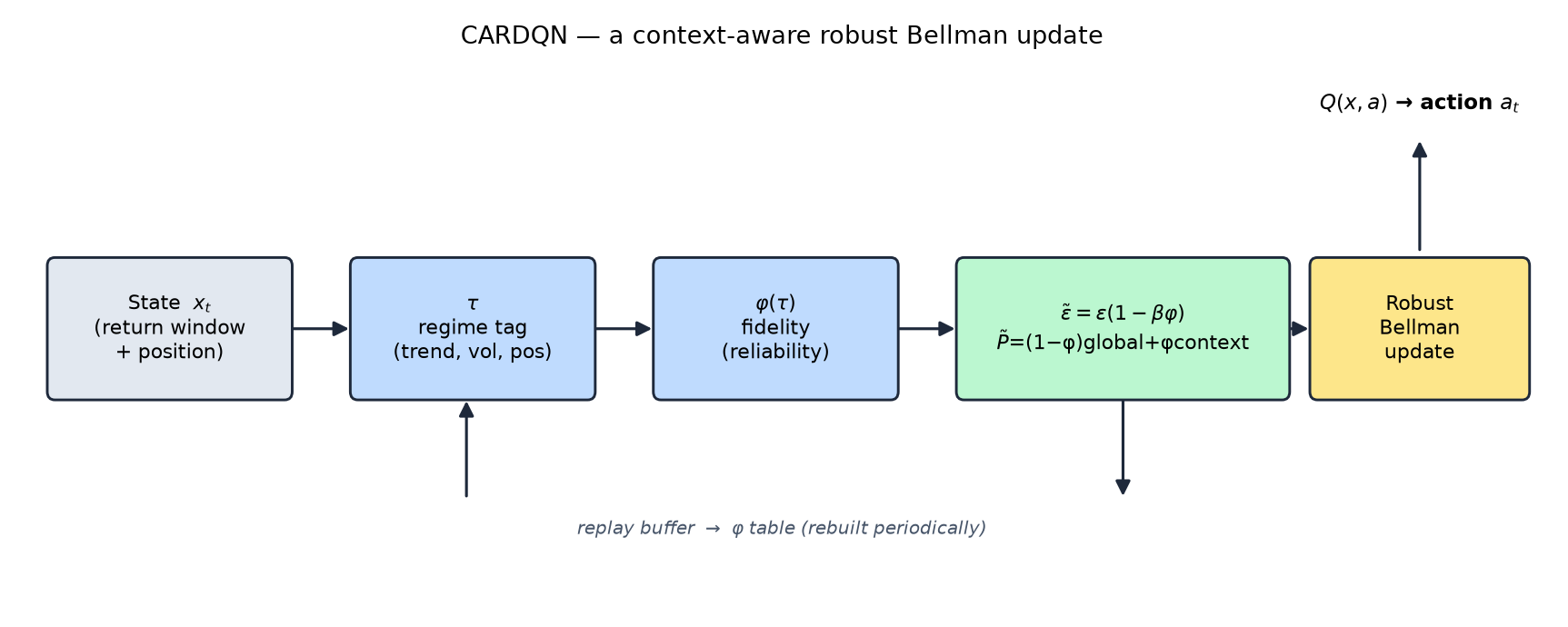
So where $\varphi\to1$ the reference becomes the regime cloud and the ball tightens; where $\varphi\to0$ it stays the safe global cloud and stays wide. Recompute cadence: the $\varphi$ table and context clouds are rebuilt from the replay buffer at most every $\varphi_{\text{refresh}}=50$ Q-updates, only once the buffer reaches $\varphi_{\text{min}}=1000$ transitions, sampling up to $20{,}000$ each time; between rebuilds $\tilde\varepsilon,\tilde P$ are just looked up (the terciles and global cloud stay frozen — only $\varphi$ and the context clouds refresh).

4.5 The target, and a proposed blend

The target is the value $Q(x,a)$ regresses toward — the Bellman RHS, built each update. CARDQN’s validated target is the robust one from §3, with the regime-adaptive ball:

A proposed but unvalidated extension blends it toward the nominal target $Q^{\text{N}}=\mathbb{E}_{\tilde P(\tau)}[r+\gamma\max_b Q]$ (no worst case), only in favorable, well-identified regimes, by a capped, fidelity-gated weight:

($q(\tau)$ scores regime favorability). Since $Q^{\text{R}} \le Q^{\text{N}}$ and $\lambda<1$, the blend stays in $[Q^{\text{R}}, Q^{\text{N}}]$ — the agent de-hedges where safe but provably never becomes optimistic. Results below are CARDQN without it.

5. How it all fits together

One training step:

tau       = context_tag(state)                              # past-only regime ∈ {1..27}
phi       = phi_table[tau]                                  # out-of-sample fidelity ∈ [0,1]
eps_tilde = eps * (1 - beta*phi)                            # tighten radius where confident
P_tilde   = (1-phi)*global_cloud + phi*context_cloud[tau]   # blend reference
target    = robust_bellman(next_states, eps_tilde, P_tilde) # worst case (Sinkhorn dual)
Q.update(state, action, target)

The $\varphi$ table and context clouds refresh every $\varphi_{\text{refresh}}$ updates (§4.4). Everything flows from the state’s past, so training and the out-of-sample backtest run identical computation — no look-ahead, no leak.

6. Does it actually work?

CARDQN (“full”) and a faithful RDQN reproduction (“off” — same code path, context layer off, a same-codebase control) train on a signature-MMD simulator, then evaluate out-of-sample on the real S&P 500, 1995–2024, proportional costs, 5 seeds, 10 episodes.

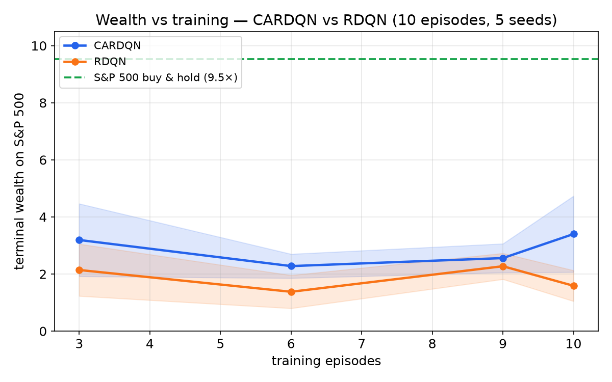
CARDQN sits above RDQN throughout. (Jagged because the deployed greedy policy is a step-function of the network — tiny training nudges flip the chosen action at pivotal days, compounding over 30 years.)

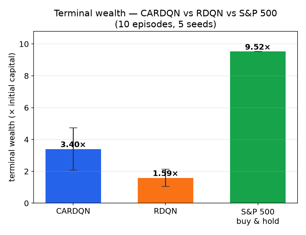
CARDQN 3.40× vs RDQN 1.59× — more than double.

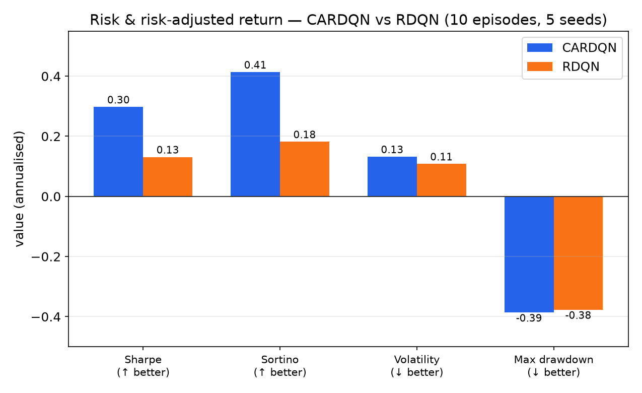
CARDQN roughly doubles RDQN’s Sharpe and Sortino (0.30 vs 0.13, 0.41 vs 0.18) at comparable volatility (0.13 vs 0.11) and drawdown (−0.39 vs −0.38). Same robustness guarantee; materially less wasted caution.

Three honest caveats: (1) nobody beats buy & hold here — every simulator-trained agent hits a sim-to-real gap (the synthetic market under-represents the S&P’s drift), separate from the robustness contribution; (2) seed variance is real — wealth is non-monotone across checkpoints (the ±std bands show it); at 30 episodes the edge is smaller but CARDQN still wins, with a smaller max drawdown; (3) research, not investment advice — it trades a simulated market.

7. Takeaways

CARDQN is a robust agent that doesn’t apply the same paranoia to every situation: tag the regime, estimate (honestly, out-of-sample) how much to trust the model there, and size the safety margin accordingly — distributionally robust optimization with a contextual twist inside a Sinkhorn-dual deep RL agent, more than doubling a robust trading agent’s terminal wealth at better risk-adjusted return. The idea isn’t finance-specific: anywhere you do robust sequential decision-making under a partially-trusted model (robotics, control, operations), “hedge hard when uncertain, commit when confident” is natural.

• Code: github.com/giuliocsr/CARDQN
• Paper: giuliocsr.github.io/papers/cardqn.pdf